Artificial Neural Network's (June 19, 2021)

Artificial Neural Network's
by Ethan Alexander Shulman (June 19, 2021)

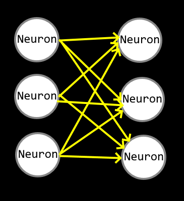
In this article I'm going to describe artificial neural networks as used in software today. The history of artificial neuralnets has gone through various stages and it could be helpful to research early models like the perceptron. Commonly called a neuralnet, artificial neural networks are an attempt to simulate biological neurons in electronics or software. The main feature being the ability to adapt and optimize towards meeting a goal or more specifically matching desired outputs to inputs. Let's begin by inspecting the inner parts of a artificial neural network and then we will walkthrough how to program a basic neuralnet in Javascript.

Structure

In the diagram to the left you can see the neurons(white) and their connections(yellow) that make up an artifical neural network. Most neuralnets used today are designed to propagate in specific forward and backward directions, the forward direction is marked by the arrows at the end of connections. This direction also gives us an input layer of neurons on the left and an output on the right.

In this diagram we have the neurons split into layers and fully connected where each neuron in one layer connects to every neuron in the next. There is also locally connected networks where neurons only connect to limited surrounding neurons. Layers in between the input/output are called hidden layers, a network with many hidden layers is called a deep neuralnetwork.

Each neuron on the left represents a real number input and each neuron on the right represents a real number output. So with the above network we would input a 3D vector and get out a 3D vector. These parts of the network also hold data, each neuron has a real value called bias and each connection has a real scalar called 'weight'. These values make up the actual programming of the network and are what you change to make the same network adapt and perform different tasks.

Simulation

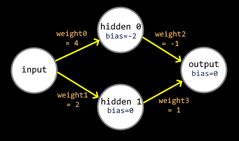
This next diagram is the network were going to simulate as an example. The simulation involves calculating the next layers neuron state values by summing all connected neuron states multiplied by weight scalars(dot product) as well as a constant bias. That summed value is passed through an activation function like tanh(x) or max(0,x) which allows advanced logic to be calculated. In this example were going to be using max(0,x) for all our hidden and output neurons, commonly called rectifier linear unit(RELU).

Let's begin writing our simulation code, were simply going to write some Javascript to run in your web browsers console. Since our network has 1 input and 1 output were going to write it as a function that takes in a input parameter and returns the network output. Below we will setup our function and initialize the constant weight and bias variables.

var hiddenBias0 = -2, hiddenBias1 = 0, outputBias = 0, weight0 = 4, weight1 = 2, weight2 = -1, weight3 = 1; function neuralnet(input)

{

var output; return output;

}

Given the process above, first we calculate hidden0 and hidden1 using input and then we calculate output using hidden0 and hidden1. Below you can see our finished neuralnet simulation function and a test which prints the neuralnets output in the console.

var hiddenBias0 = -2, hiddenBias1 = 0, outputBias = 0, weight0 = 4, weight1 = 2, weight2 = -1, weight3 = 1; function neuralnet(input)

{

//calculate hidden layer from input

var hidden0 = Math.max(0, input*weight0 + hiddenBias0), hidden1 = Math.max(0, input*weight1 + hiddenBias1)

;

//calculate ouput from hidden

var output = Math.max(0, hidden0*weight2 + hidden1*weight3 + outputBias)

;

return output;

}

for

(

var x = 0; x < 1.01; x += 0.1) console.log(x.toFixed(2)

"(X) - "

+neuralnet(x).toFixed(2)

"(NN)"

)

;

To run the code open your web browser console either by pressing F12 or selecting 'Inspect Element' in the menu and open the 'console' tab. Copy the code above, paste it into the console and press enter to run it. After running it you should see the following output in your console.

0.00(X) - 0.00(NN) 0.10(X) - 0.20(NN) 0.20(X) - 0.40(NN) 0.30(X) - 0.60(NN) 0.40(X) - 0.80(NN) 0.50(X) - 1.00(NN) 0.60(X) - 0.80(NN) 0.70(X) - 0.60(NN) 0.80(X) - 0.40(NN) 0.90(X) - 0.20(NN) 1.00(X) - 0.00(NN)

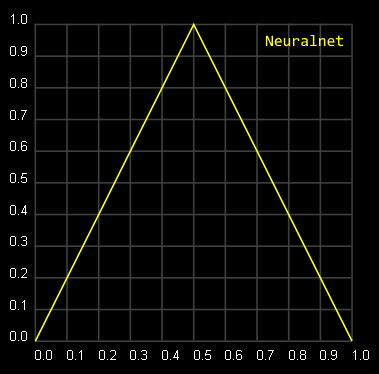
If you graph these values you will notice our neuralnet is plotting a triangle wave!

Learning
Above we established what an artificial neural network is made up of and how to simulate one. But we only ran a fixed neuralnet that had preset weights and biases, the real challenge is programmatically determining the weights and biases to match our desired goal. This is commonly called learning, training, optimizing or evolving. The many names for the process come from the variety of ways there are to build the weights and biases. The big popular method that has made neuralnetworks so popular is called gradient descent and is built off automatic differentiation. Another family of methods is genetic algorithms.

Neural network learning is a giant topic and I will cover it in more depth in a later article.

Thanks for Reading!
If you have any questions feel free to reach out to me at xaloezcontact@gmail.com.